Solutions of Exercise 5.1

Consider the control system in Fig. 41, where \(v(t)\) is a sinusoidal disturbance \(v(t) = \sin(\omega t)\).

Fig. 41 Block diagram of the control system

The proportional controller has a positive gain, that is, \(K > 0\).

1. Compute, as a function of \(K\), the absolute value of the sensitivity function at \(\omega = 1\) rad/s.

2. Determine for what values of \(K\) the disturbance \(v(t)\) gets attenuated[1] by a factor of \(9\) at the frequency \(\omega= 1\) rad/s.

If necessary, use the asymptotic Bode plot of \(G(s)\) shown in Fig. 42.

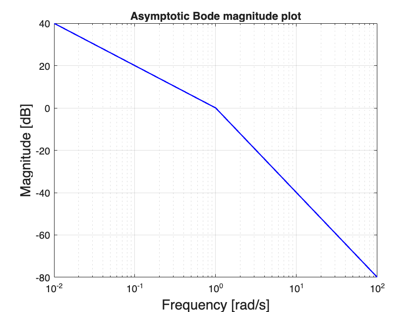
Fig. 42 Magnitude Bode plot of \(G(s)\)

---

Solution

Question 1

From Lecture 7, we know that the sensitivity function \(S(s)\) is the transfer function between \(V(s)\) and \(Y(s)\):

\[ S(s) \equiv \frac{Y(s)}{V(s)} = \frac{1}{1 + G_o(s)} = \frac{1}{1 + K \frac{1}{s^2 + s}} = \frac{s^2 + s}{s^2 + s + K} \]

Note that \(S(s)\) is stable for any \(K>0\) (Routh-Hurwitz criterion).

We can now compute its modulus (absolute value) at \(\omega = 1\) rad/s

\[ \lvert S(i \omega) \lvert = \left\lvert\frac{ (i \omega)^2 + i \omega}{(i \omega)^2 + i \omega + K} \right\lvert \]

Knowing that \(i^2 = -1\) and that \(\omega = 1\) rad/s, we get

\[ \lvert S(i \omega) \lvert = \left\lvert \frac{ -1 + i }{K - 1 + i } \right\lvert \]

We now multiply and divide the denominator by \((K - 1) - i\), to make the denominator real

\[ \lvert S(i \omega) \lvert = \left\lvert \frac{-1 + i }{(K - 1 + i) \cdot \frac{K - 1 - i}{K - 1 - i}} \right\lvert = \left\lvert \frac{ (-1 + i)(K - 1 - i)}{ (K-1)^2 - i^2 } \right\lvert = \left\lvert \frac{-K + 1 + i+ i K - i - i^2}{K^2 - 2K + 1 + 1} \right\lvert \]

Let’s now isolate the real part of the numerator from the imaginary part

\[ \lvert S(i \omega) \lvert = \left\lvert \frac{-K + 2 + i K }{K^2 - 2K + 2} \right\lvert = \left\lvert \underbrace{\frac{-K + 2}{K^2 - 2K + 2}}_{\text{Real}} + i \underbrace{\frac{K}{K^2 - 2K + 2}}_{\text{Imaginary}} \right\lvert \]

The modulus of this complex number is given by the square-root of the real part squared plus the imaginary part squared:

\[ \lvert S(i \omega) \lvert = \sqrt{\left(\frac{-K + 2}{K^2 - 2K + 2}\right)^2 + \left(\frac{K}{K^2 - 2K + 2} \right)^2} = \sqrt{\frac{(-K+2)^2 + K^2}{(K^2 - 2K + 2)^2}} = \sqrt{\frac{2\cancel{(K^2 - 2K + 2)}}{(K^2 - 2K + 2)^{\cancel{2}}}} = \sqrt{\frac{2}{\lvert K^2 - 2K + 2 \lvert}} \]

We further notice that \(K^2 - 2K + 2 = (K-1)^2 + 1\) which is always positive (it’s the sum of two squares). The expression of \(\lvert S(i \omega) \lvert\) becomes

(16)\[ \lvert S(i \omega) \lvert = \sqrt{ \frac{2}{(K-1)^2 + 1}} \]

Question 2

Since \(S(s)\), the Frequency Response Theorem tells us that \(\lvert Y(i \omega)\lvert = \lvert S(i \omega) \lvert \cdot \lvert V(i \omega) \lvert\) where, in our case, \(\omega = 1\). The attenuation factor of \(4\) is achieved if

\[ \lvert S(i 1) \lvert \leq \frac{1}{9} \]

From (16), we can write

\[ \sqrt{\frac{2}{(K-1)^2 + 1}} \leq \frac{1}{9} = \frac{1}{\sqrt{81}} \]

This is achieved if the denominator is at least \(81\) times larger than the numerator:

\[ (K-1)^2 + 1 \geq 81 \cdot 2 \]

Moving the term \(+1\) on the right hand side, we conclude that the inequality is solved by \((K-1)^2 \geq 161\), i.e., \(K - 1 \leq -\sqrt{161} \cup K - 1 \geq \sqrt{161}\).

The first interval, \(K \leq 1 - \sqrt{161} < 0\) needs to be discarded because \(K > 0\). The set of \(K\) that satisfy the disturbance attenuation requirement is therefore

\[ \boxed{K \geq 1 + \sqrt{161} \approx 14} \]

Alternative solution via Bode plots

The problem could have been solved very easily with Bode plots. Even though approximate, this solution is the suggested one.

We start by noting that \(G_o(s) = G(s)\) for \(K=1\). For this specific \(K\), we can sketch the sensitivity function’s magnitude plot according to:

(17)\[\begin{split} \lvert S(i \omega) \lvert_{\text{dB}} \approx \begin{dcases} - \lvert G_o (i \omega) \lvert_{\text{dB}} & \text{where } \lvert G_o (i \omega) \lvert_{\text{dB}} < 0\text{dB} \\ 0 ~\text{dB} & \text{where } \lvert G_o (i \omega) \lvert_{\text{dB}} > 0 \text{dB} \end{dcases} \end{split}\]

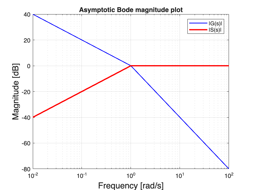
Fig. 43 Sketch of the sensitivity function’s magnitude plot according to the asymptotic Bode plot of \(G_o(s)\) for \(K=1\).

Clearly, for \(K=1\), \(\lvert S(i 1)\lvert = 0 \text{dB}\). In order to ensure an attenuation factor of \(9\), we must have that \(\lvert S(i 1)\lvert \leq 9\) or, in decibels, \(\lvert S(i 1)\lvert_{\text{dB}} \leq -19 \text{dB}\).

To achieve this, according to (17), we must find \(K\) so that \(\lvert G_o(i1) \lvert_{\text{dB}} > -19 \text{dB}\). Because for \(K=1\) the magnitude of the open-loop transfer function in \(\omega=1\) is \(\lvert G_o(i \omega)\lvert_{\text{dB}} \approx 0 \text{dB}\), \(K\) must be larger than \(19\) dB. That is, \(K > 9\).

Note

This result is quite different from that derived in the analytical solution of Question 2. The reason is that in Fig. 43 we used the asymoptotic Bode diagrams, which are inaccurate near the open-loop poles (which, in our case, sadly happen to be in \(s=-1\), at \(\omega = 1\)).

Curious to see a proof? See Plotting the exact Sensitivity function!

This solution is however perfectly acceptable in the context of our course.

---

[1]

That is, the effect of \(v(t)\) on the output \(y(t)\) is \(\frac{1}{9}\) of the maximum amplitude of \(v(t)\), in this case \(1\). In this case, we say that the closed-loop achieves an attenuation factor of \(9\) for disturbances at frequency \(\omega = 1\).