Solutions of Exercise 2.2

We want to control the angular position of a DC motor. The transfer function between the applied voltage and the position is

\[ G(s) = \frac{10}{s(s+10)} \]

We adopt a proportional controller:

\[ F(s) = K \]

1. For which values of \(K\) is the closed-loop stable?

2. If the reference signal is \(\theta_{ref}(t) = R \cdot \textrm{step}(t)\), for what values of \(K\) the steady-state output error is less than \(1\%\)?

---

Solution

Question 1

We start by computing the closed-loop transfer function:

\[ G_c(s) = \frac{K \cdot G(s)}{1 + K \cdot G(s)} = \frac{10 K}{s^2 + 10 s + 10 K} \]

Then, similar to Exercise 1.3, we analyze how the poles of \(G_c(s)\) change as a function of \(K\).

\[ s^2 + 10s +10K = 0 \]

The discriminant is \(\Delta = 100 - 40 K\).

Case \(\Delta > 0\)

If \(K \leq 2.5\), the discriminant is positive (\(\Delta > 0\)), which means we have two real solutions

\[ s = \frac{-10 \pm \sqrt{100 - 40K}}{2} = -5 \pm \sqrt{25 - 10K} \]

The real part of the poles is strictly negative as long as \(\sqrt{25 - 10K} \leq 5\), that is, \(0 < K \leq 2.5\).

Case \(\Delta < 0\)

If \(K > 2.5\) the discriminant is negative, hence we have two complex-conjugate solutions

\[ s = \frac{-10 \pm i \sqrt{\lvert \Delta \lvert}}{2} = -5 \pm i \sqrt{\frac{\lvert \Delta \lvert}{4}} \]

The real part is negative and independent of \(K\). Therefore, for any \(K > 2.5\) the closed-loop is stable.

Solution to question 1

Any \(K > 0\) makes the closed-loop stable.

We can double-check this result looking at the root locus of the system.

s = tf('s');
G = 10/(s*(s+10));
rlocus(G); hold on; 

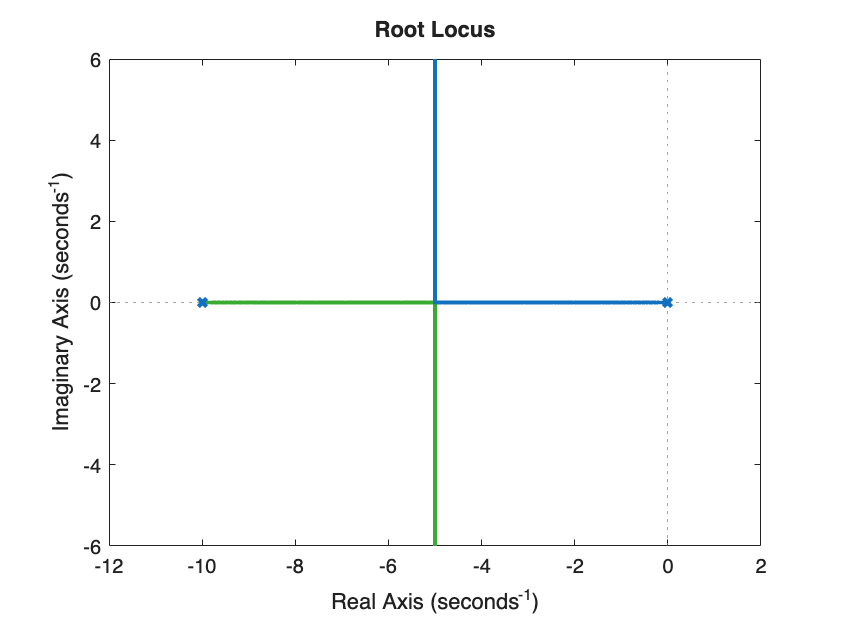
As can be seen, the closed-loop poles are always located in the left-hand half-plane.

Alternative solution with the Routh criterion

Hint

Checking the stability of a transfer function is usually easier with the Routh criterion, especially when the system is of order \(n \geq 2\) and/or contains parameters (in this case, \(K\)).

The characteristic polynomial, i.e., the denominator of \(G_c(s)\), is

\[ s^2 + 10 s + 10 K = 0 \]

Applying the formula seen during the lectures, the Routh-Hurwitz table reads

\( \begin{array}{cc} 1 & 10K \\ 10 & 0 \\ \hline 10K & 0 \end{array} \)

For stability, all elements in the first column must be strictly positive:

\( \begin{cases} 1 > 0 \\ 10 > 0 \\ 10 K > 0 \implies K > 0 \end{cases} \)

Thus, the system is stable for \(K > 0\).

Question 2

We now restrict ourselves to the case \(K > 0\), where the closed-loop is stable. Thanks to the stability of the closed-loop, we can apply the Final Value Theore (where \(\Theta_{ref}(s) = \frac{R}{s}\))

\[ \lim_{t \to \infty} \theta(t) = \lim_{s \to 0} s \left( G_c(s) \Theta_{ref}(s) \right) = \lim_{s \to 0} s \left( \frac{10 K}{s^2 + 10 s + 10 K} \frac{R}{s} \right) = \frac{10K}{10 K} = R \]

The steady-state error is \(e(\infty) = \theta_{ref}(\infty) - \theta(\infty) = R - R = 0\) for every value of \(K > 0\).