Exercise 1.2#
Analysis ∙ Linear dynamical systems
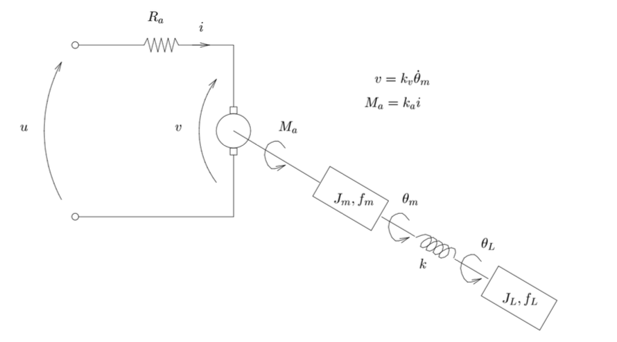
Fig. 3 Schematic of the motor with a load (courtesy of Exercise Manual for Automatic Control)#
Assume that the DC-motor in Exercise 1.1 is running a load attached to an elastic axis, as in the figure above. Let \(k\) be the axis’ spring constant, and let \(J_L\) be the moment of inertia of the load.
Write the transfer function between the input voltage \(u\) and the angle \(\theta_L\).
Hint
To retrieve the governing equations, you can write the balance of momentum of both the load:
where, \(J_L \ddot{\theta}_L\) is the motor inertia equaling the sum of the friction (\(-f_L \dot{\theta}_L\)) and of the elastic force \( k (\theta_L - \theta_m)\), and of the motor
where the motor inertia (\(J_m \ddot{\theta}_m\)) equals the sum of the friction term (\(-f_m \dot{\theta}_m\)), the elastic force (\( k (\theta_L - \theta_m)\)), and the motor torque (\(k_a i\)).