Exercise 3.3#

Fig. 15 Block diagram of the closed loop#
A system \(G(s)\) is controlled using a feedback with a proportional controller according to Fig. 15. \(G(s)\) has no unstable pole, that is, no pole with positive real part.
In Fig. 16, the Nyquist diagram of four different systems \(G(s)\) are reported. Find, for each of these systems, the values of \(K\) for which the closed-loop is stable.
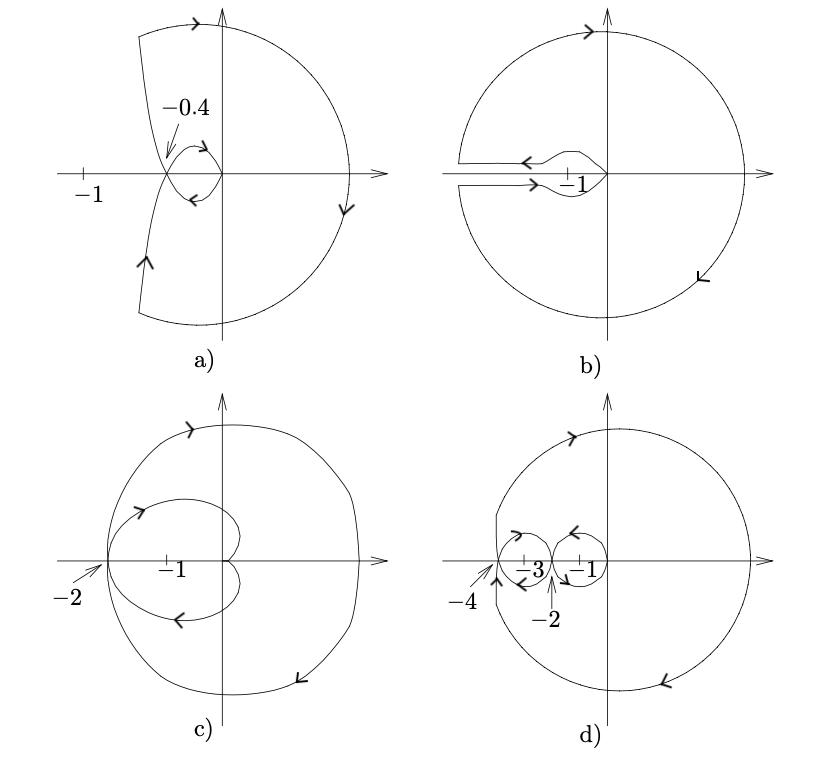
Fig. 16 Nyquist plots of \(G(s)\)#