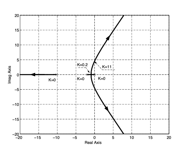
Exercise 2.1

Analysis ∙ Feedback control

Fig. 9 Root Locus plot

We want to design a proportional controller \(F(s)=K\) for a tooling machine. In the Root Locus plot, the poles of the closed-loop system \(G_c(s) = \frac{F(s)G(s)}{1 + F(s)G(s)}\) are drawn as a function of the controller gain \(K\).

Use the Root Locus plot to specify what values of \(K\) have been used to generate the step responses depicted in the figure below.

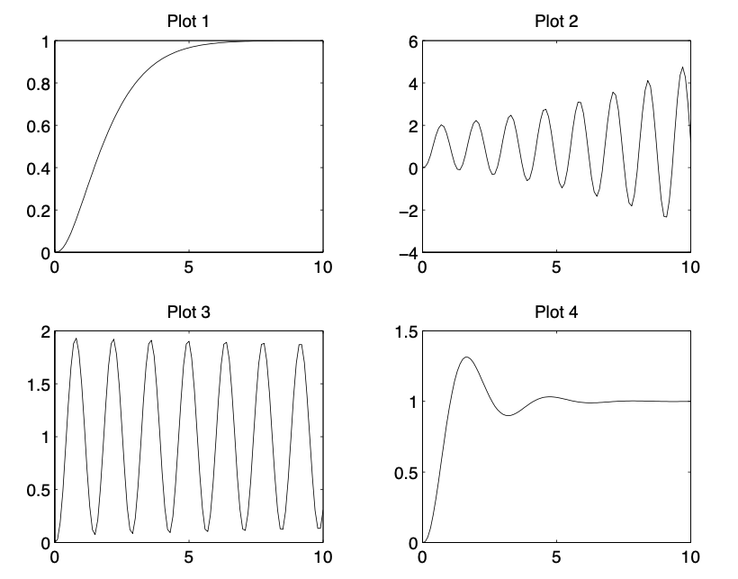
Fig. 10 Closed-loop step responses