Exercise 1.4#
Analysis ∙ Linear dynamical systems
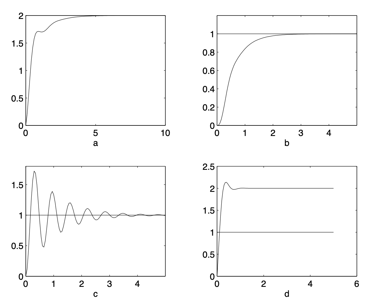
Fig. 7 Step responses to consider (courtesy of Exercise Manual for Automatic Control)#
Pair each step response in the plot above with the correct transfer function from the list below:
\(G_1(s) = \frac{100}{s^2 + 2s + 100}\)
\(G_2(s) = \frac{1}{s+2}\)
\(G_3(s) = \frac{10 s^2 + 200s + 2000}{(s+10)(s^2 + 10s + 100)}\)
\(G_4(s) = \frac{100}{s^2 + 10s + 100} \cdot \frac{2}{s+2}\)
\(G_5(s) = \frac{100}{s^2 + 10s + 100} + \frac{2}{s+2}\)
\(G_6(s) = \frac{100}{s^2 - 10s + 100} \cdot \frac{1}{s+2}\)
Useful formulas to compute the damping ratio and natural frequency of complex-conjugate eigevalues are reported in the Useful formulas.