Exercise 5.2

Analysis ∙ Robustness of feedback controllers

Fig. 44 Block diagram of the control system

The controller \(F(s) = \frac{s+10}{s}\) was designed assuming that the system \(G^0(s)\) was identical to the model \(G(s) = \frac{1}{s+10}\). In Fig. 45, the nominal open-loop transfer function \(G_o(s) = F(s) \cdot G(s)\).

1. Sketch the nominal complementary sensitivity function \(T(s)\) using the sketching rules discussed in Lecture F7.

Unfortunately, there’s a mismatch between the real system \(G^0(s)\) and its model \(G(s)\). In fact

\[ G^0(s) = G(s) \left( 1 + \Delta(s) \right) \]

where the multiplicative uncertainty \(\Delta(s)\) does not have any pole in the right-hand half plane, but is not known. We know, however, an upper bound for its amplitude

(18)\[ \lvert \Delta(i \omega) \lvert \leq \frac{0.9}{\sqrt{1 + \omega^2}} = \left\lvert \frac{0.9}{1 + i \omega} \right\lvert \]

2. Does the feedback controller \(F(s)\), implemented as in Fig. 44, guarentee the closed-loop stability for \(G^0(s)\) despite the uncertainty?

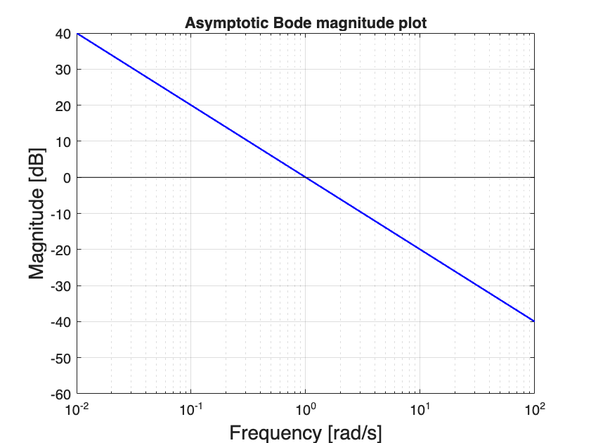
Fig. 45 Magnitude Bode plot of the nominal open-loop transfer function \(G_o(s)\).