Solutions of Exercise 7.4#
For the system \(G(s) = 5 \frac{s + 7}{(s + 2)^3}\) a colleague of yours has designed the following feedback controller:
The Bode plots of the open-loop transfer function \(G_o(s)\) are reported in Fig. 64,
Suggest a range of possible sampling frequencies at which the discretized controller should operate.
Pick a value of the sampling frequency, and compute the (algebraic) discretized control law using any method of choice (Forwad Euler, Backward Euler, Trapezoidal rule).
What is the loss of phase margin? Is the residual phase margin still sufficient?
s = tf('s');
G =  5 * (s + 7) / (s+2)^3;
F = 10 * (s + 2) / (s+7);
bode(F*G); grid on; box on;
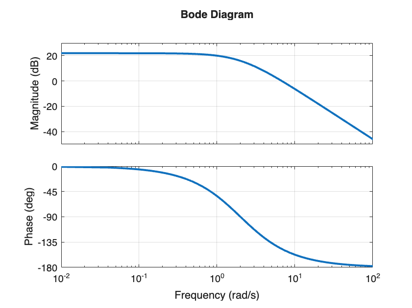
Fig. 64 Bode plot of the open-loop transfer function \(G_o(s) = F(s) G(s)\).#
Solution#
Question 1#
From Fig. 64, the crossover frequency is \(\omega_c \approx 6.5\) rad/s. In Hz, this is \(f_{c} = \frac{\omega_c}{2 \pi} \approx 1\) Hz. According to the rule-of-thumb presented during the lectures, a good value of the sampling frequency \(f_s\) is in the range
Therefore, \(f_s \in [20, 50]\) Hz. This ensures that the sampling is fast enough for the controller (i.e., it doesn’t lead to large losses of phase margins), while not too fast fast (which would lead to unreasonably expensive hardware and to actuator’s wear-and-tear).
Common pitfall
A common error is to invoke the Nyquist-Shannon Theorem and answer \(f_s > 2 f_c\). This solution is wrong, because the error signal \(e(t)\) being sampled is not band-limited to \(f_c\). The error has indeed frequency components at frequencies higher than \(f_c\), therefore this theorem cannot be applied![1]
Question 2#
Let’s pick \(f_s = 25\) Hz, meaning that the sampling time is \(T = \frac{1}{25} = 0.04\). We will use the Forward Euler formula (\(\alpha = 0\)), and replace
into the continuous-time controller
Apply this substitution we actually translate the control law in the discrete-time domain:
Multiplying both sides by \((25 - 18q^{-1})\), we get
Recalling that \(q^{-1}\) is the time-shift operator, we can finally get the algebraic, discrete-time control law by isolating \(u_k\):
In practice, this control law can be implemented by, e.g., the following C function invoked every \(T=0.04\) seconds:
float control_law(float u_prev, float e_prev, float e_current)
{
    return 0.72f * u_prev
         + 10.0f * e_current
         - 9.2f  * e_prev;
}
Curious to see how this kind of controllers can be implemented on Arduino? Check out this code!
Question 3#
The phase loss due to the discretization procedure is
The phase margin achieved by the continuous-time controller was (see Fig. 64) approximately \(\varphi \approx 33\).
The new phase margin is \(33^\circ - 7.5^\circ = 25.5^\circ\). While rather low, this phase margin is still enough to guarantee closed-loop stability, at the price of rather large oscillations.