Solutions of Exercise 3.2

A vehicle is characterized by the following transfer function, which relates the throttle input \(U(s)\) to the velocity \(Y(s)\),

\[ G(s) = \frac{s+10}{(s+1)^2(s+5)} \]

We need to design a controller that regulates the speed of the vehicle.

1. Start by designing a proportional controller \(F(s) = K\). For what values of \(K > 0\) is the closed-loop stable? How does the closed-loop performance change when \(K\) is changed?

2. Consider now \(K=10\). Compute the gain margin \(A_m\) and the phase margin \(\varphi_m\).

Hint

To check the stability of the closed-loop transfer function \(G_c(s)\), you can use the root locus (plotted with MATLAB), or the Routh-Hurwitz criterion.

---

Solution

Question 1

Since the order of the closed-loop transfer function \(G_c(s) = \frac{F(s) G(s)}{1 + F(s) G(s)}\) is three, we can’t easily provide an analytical solution. We therefore inspect the root locus.

% Check if the `asymptotic_bode` and `rlocus_arrows` functions are available, otherwise download them from the github URLs.
if ~exist('asymptotic_bode')
    urlwrite('https://raw.githubusercontent.com/bonassifabio/1RT485/refs/heads/main/book/res/matlab/asymptotic_bode.m', 'asymptotic_bode.m');
end
if ~exist('rlocus_arrows')
    urlwrite('https://raw.githubusercontent.com/bonassifabio/1RT485/refs/heads/main/book/res/matlab/rlocus_arrows.m', 'rlocus_arrow.m');
end

s = tf('s');
G =  1 * (s + 10) / ((s + 1)^2 * (s + 5));

rlocus_arrows(G); % A convenient wrapper of rlocus that add arrows and relevant points to the root locus plot.

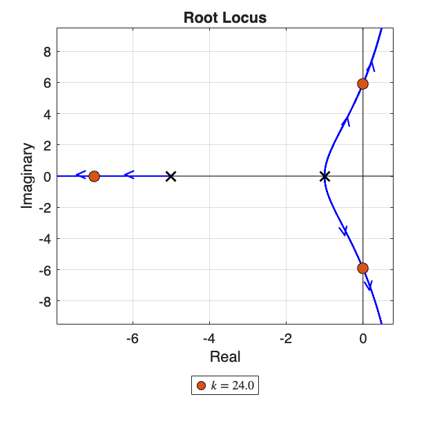
From the root locus, we can see that the closed-loop poles are stable for \(K < 24\).

Alternative solution: the Routh criterion

To check the stability of \(G_c(s)\) we can apply the Routh criterion as done in the Solutions of Exercise 2.5.

To do so, let’s first compute \(G_c(s)\):

\[ G_c(s) = \frac{F(s)G(s)}{1+F(s)G(s)} = \frac{\frac{K(s+10)}{(s^2 + 2s + 1)(s+5)}}{1 + \frac{K(s+10)}{(s^2 + 2s + 1)(s+5)}} = \frac{K(s+10)}{s^3 + 7s^2 + (11+ K)s + 10K + 5} \]

The characteristic polynomial is the denominator of \(G_c(s)\), i.e., \(\Phi = s^3 + 7s^2 + (11 + K)s + (10K + 5)\). The Routh-Hurwitz table therefore reads

\[\begin{split} \begin{array}{cc} 1 & 11 + K \\ 7 & 10K + 5\\ \hline \frac{72 - 3K}{7} & 0 \\ 10 K + 5 \end{array} \end{split}\]

According to the Routh criterion, \(G_c(s)\) is stable if and only if all the elements on the first column are positive. Note that \(1>0\) and \(7>0\) for any \(K\), therefore we will omit them.

\[\begin{split} \begin{dcases} 72 - 3K > 0 \\ 10K + 5 > 0 \end{dcases} \quad \rightarrow \quad \begin{dcases} K < 24 \\ K > -0.5 \end{dcases} \end{split}\]

Therefore, \(\boxed{0 < K < 24}\). Note that the lower limit has been limited to \(0\) because the text of the exercise specified \(K>0\).

Question 2

Phase margin

Let’s start by computing the phase margin, which is defined as

\[ \varphi_m = 180^o + \angle G_o(i \omega_c) \]

where \(G_o(s) = F(s) G(s)\) is the open-loop transfer function and \(\omega_c\) is the critical frequency, that is, the frequency where the open loop transfer function has unitary amplitude, \(\lvert G_o(i \omega_c) \lvert = 1\). Remember that \(G_o(i \omega)\) is a complex number!

\[ G_o(s) = 10 \frac{s + 10}{(s+1)^2(s+5)} \]

To compute \(\omega_c\) we replace \(s = i \omega\) for different values of \(\omega\), until we find a value where the modulus of \(G_o(i \omega)\) is approximately \(1\).

Go_modulus = @(w) abs(10 * (1i * w + 10) / ((1i * w + 1)^2 * (1i * w + 5)));

Go_modulus(1)
Go_modulus(10)
Go_modulus(4)

ans = 9.8547

ans = 0.1252

ans = 0.9894

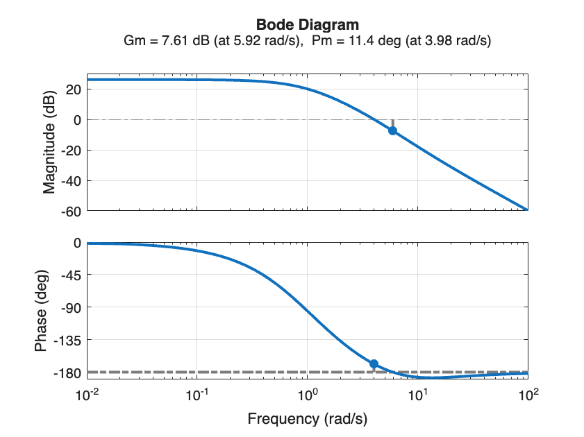
Therefore \(\omega_c \approx 4\) rad/s.

Note

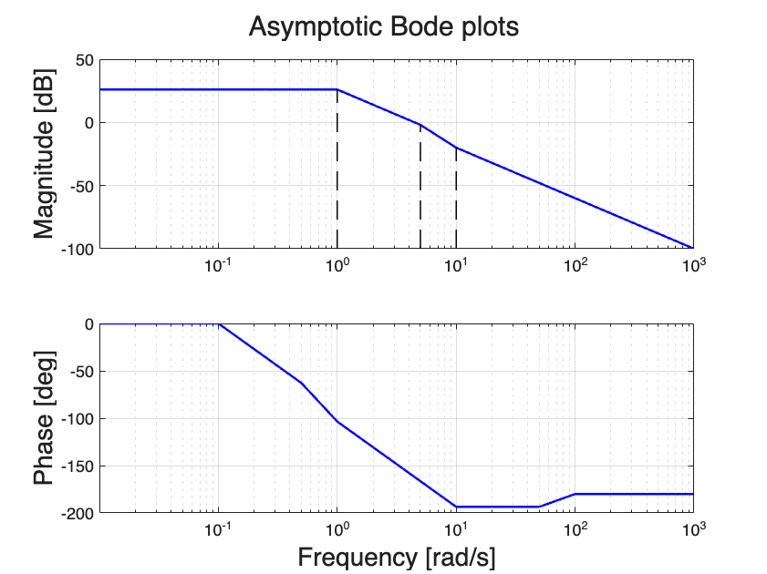
You can also find the critical frequency from the Bode diagram, as the interception between the plot of \(\lvert G_o(i \omega) \lvert_{\text{dB}}\) and the 0dB axis!

figure; asymptotic_bode(10 * G)

We can now evaluate the phase margin as

\[ \varphi_m = 180 + \angle G_o(i 4) \]

% We create a function that computes the angle of Go given the frequency omega
% We use the mod function to convert the angle to the range [-360, 0]
Go_phase = @(w) mod(rad2deg(angle(10 * (1i * w + 10) / ((1i * w + 1)^2 * (1i * w + 5)))), 360) - 360;

phase_margin = 180 + Go_phase(4)   % Conver the angle from radians to degrees

phase_margin = 11.2141

While a phase margin of \(11^\circ\) is bigger than \(0^\circ\), so it is enough to guarantee the closed-loop stability, in practical applications it is too low to be accepted.

• If \(\varphi_m > 90^\circ\), the dominant closed-loop pole is real valued and stable.

• If \(0^\circ < \varphi_m < 90^\circ\), the dominant closed-loop poles are complex-conjugate, with damping coefficient \(\xi = \cos(\varphi_m)\), see Useful formulas.

• If \(\varphi_m \leq 0^\circ\), the system is unstable.

Warning

A phase margin below \(30^\circ\) indicates that the dominant poles have a low damping coefficient. In general, the phase margin should be at least \(45^\circ\) for adequate closed-loop performance.

Gain margin

We can then proceed computing the gain margin, which is defined as

\[ A_m = \frac{1}{\lvert G_o(i \omega_p) \lvert} \]

or, in decibels,

\[ A_m = -\lvert G_o(i \omega_p) \lvert_{\text{dB}} \]

Here \(\omega_p\) is the phase crossover frequency, i.e., the frequency at which the phase plot first crosses the \(-180^\circ\) axis. To find \(\omega_p\) we need to solve

(5)\[ \angle G_o(i \omega) := \varphi(0) + \sum_{i} \textrm{atan} \left( \frac{\omega}{p_i} \right) - \sum_{i} \textrm{atan} \left( \frac{\omega}{z_i} \right) = -180^\circ \]

The initial phase \(\varphi(0)\) is \(0^\circ\) if the static gain is positive, decremented by \(90^\circ\) for each pole in the origin and incremented by \(90^\circ\) for each zero in the origin. In (5), \(p_i\) is the \(i\)-th pole of \(G_o(s)\) and \(z_i\) is the \(i\)-th zero.

To compute \(\omega_p\) we try replacing some candidate value until we find a value where \(\angle(G_o(i \omega)) = -180^\circ\). Note that the phase might cross the \(-180^\circ\) axis multiple times, and we must be sure that we get the smallest possible of such values. The easiest way to find a reasonable value is to sketch the asymptotic Bode diagram (see above).

It is apparent that the phase is crossing is somewhere between \(4\) rad/s and \(10\) rad/s. To find the exact value, we try evaluate \(\angle G_o(i \omega)\) in that range

Go_phase(5)
Go_phase(7)
Go_phase(6)

ans = -175.8151

ans = -183.2101

ans = -180.3060

Therefore, \(\omega_p \simeq 6\) rad/s. We can finally evaluate the gain margin as

Am = 1 / Go_modulus(6)

Am = 2.4780

20 * log10(Am)

ans = 7.8819

The gain margin is \(A_m \simeq 2.5 \simeq 7.8 \text{ dB}\). Since it is bigger than \(1\) (i.e. \(0\) dB), the closed-loop is stable.

We can confirm our results using MATLAB’s margin command.

figure;
margin(10 * G); grid on;