Dominant pole approximation

In this page, we show how to determine the dominant pole approximation of a third-order system having a real pole (\(s=-\gamma\)) and two complex-conjugate ones (\(s = -\alpha \pm i \beta\)). Let this higher order system be

\[ G(s) = \frac{\mu}{(s + \gamma)(s+ \alpha + i \beta)(s + \alpha - i \beta)} \]

We assume that all the poles are on the left-hand side (\(\alpha >0\), \(\gamma > 0\)).

According to the page Useful formulas, we need to check whether \(\gamma < \sqrt{\alpha^2 + \beta^2}\) or \(\gamma > \sqrt{\alpha^2 + \beta^2}\).

Case 1: The real pole is dominant

If \(\gamma < \sqrt{\alpha^2 + \beta^2}\), the real pole is dominant because its closer to the origin. In this case, we can obtain the dominant pole approximation by replacing \(s=0\) into the complex conjugate poles

\[ \boxed{\tilde{G}_1(s)} = \frac{\mu}{s + \gamma} \cdot \frac{1}{\alpha^2 + \beta^2} = \boxed{\frac{\tilde{\mu}_1}{s + \gamma}} \quad \text{ where } \tilde{\mu}_1 = \frac{\mu}{\alpha^2 + \beta^2} \]

The adjustment of \(\mu\) to \(\tilde{\mu}_1\) makes the static gain of \(\tilde{G}_1(s)\) the same as that of \(G(s)\).

Case 2: The complex-conjugate poles are dominant

If \(\gamma > \sqrt{\alpha^2 + \beta^2}\), the complex-conjugate poles are dominant as they are closer to the origin (they have a smaller modulus). In this case, we can obtain the dominant pole approximation by replacing \(s=0\) into the real pole

\[ \boxed{\tilde{G}_2(s)} = \frac{\mu}{(s+ \alpha + i \beta)(s + \alpha - i \beta)} \cdot \frac{1}{\gamma} = \frac{\tilde{\mu}_2}{ (s+ \alpha + i \beta)(s + \alpha - i \beta)} = \boxed{\frac{\tilde{\mu}_2}{s^2 + b s + c}} \]

where:

• \(\tilde{\mu}_2 = \frac{\mu}{\gamma}\) adjusts the static gain of \(\tilde{G}_2(s)\) to make it identical to that of \(G(s)\)

• \(b = 2 \alpha \)

• \(c = \alpha^2 + \beta^2\)

Exploratory example

Below these approximations are reported for a system with the specified values of \(\alpha\), \(\beta\), and \(\gamma\), while \(\mu\) is computed so that the static gain of \(G(s)\) is \(1\) for ease of visualization.

Try out

Open this page in Binder and try to change the values of \(\alpha\), \(\beta\), and \(\gamma\), and reflect on the following points:

• What is the dominant pole in this case?

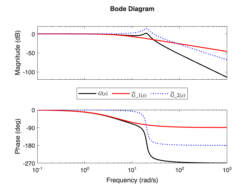
• Does the Bode plot of the dominant pole approximation resemble that of \(G(s)\)?

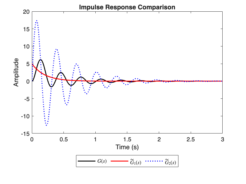
• In your specific case, do the impulse and step response look better for \(G_1(s)\) or \(G_2(s)\)?

• Is the settling time accurate?

Note

The dominant pole approximation is usually good if \(\gamma\) is at least \(5 \div 10\) smaller/larger than \(\sqrt{\alpha^2 + \beta^2}\). In this case, the poles are well separated and the approximation becomes more accurate!

% Real pole is s = - gamma
gamma = 5; % gamma > 0
% Complex conjugate poles are s = -alpha + i beta
alpha = 2; % alpha > 0
beta = 20; % beta > 0

Show code cell source

Hide code cell source

s = tf('s');
G = gamma * (alpha^2 + beta^2) / ((s + gamma)* (s^2 + 2 * alpha * s + alpha^2 + beta^2));
G1 = gamma / (s + gamma);
G2 = (alpha^2 + beta^2) / (s^2 + 2 * alpha * s + alpha^2 + beta^2);

figure; 
pzmap(G); grid on; 

if exist('OCTAVE_VERSION', 'builtin') == 0
    % MATLAB-specific plot settings
    set(get(gca, 'Responses'), 'MarkerSize', 20, 'LineWidth', 2); % Set pole marker size
end
title('Poles of G(s)');

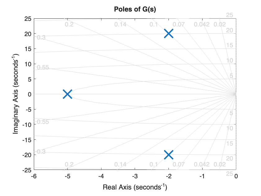
What is the dominant pole?

Show code cell source

Hide code cell source

if gamma < sqrt(alpha^2 + beta^2)
    str = sprintf('Dominant pole: s = -%.2f. G1(s) is the dominant pole approximation of G(s).', gamma);
    style_g1 = 'r-';
    style_g2 = 'b:';
else
    str = sprintf('Dominant poles: s = -%.2f +/- i %.2f. G2(s) is the dominant pole approximation of G(s).', alpha, beta);
    style_g1 = 'r:';
    style_g2 = 'b-';
end
disp(str);

Dominant pole: s = -5.00. G1(s) is the dominant pole approximation of G(s).

Bode plots comparison

Show code cell source

Hide code cell source

figure;
bodeplot_universal(G, 'k-', G1, style_g1, G2, style_g2);
legend('$G(s)$', '$\tilde{G}_1(s)$', '$\tilde{G}_2(s)$', 'Interpreter', 'latex', 'Location', 'southoutside', 'Orientation', 'horizontal');

Step and impulse response comparison

Show code cell source

Hide code cell source

T_end = 6 / min(gamma, alpha);
t = 0:1e-4:T_end;
[y, ~] = impulse(G, t);
[y1, ~] = impulse(G1, t);
[y2, ~] = impulse(G2, t);
figure; hold on; box on;
title('Impulse Response Comparison');
plot(t, y, "k-");
plot(t, y1, style_g1);
plot(t, y2, style_g2);
legend('$G(s)$', '$\tilde{G}_1(s)$', '$\tilde{G}_2(s)$', 'Interpreter', 'latex', 'Location', 'southoutside', 'Orientation', 'horizontal');
xlabel('Time (s)');
ylabel('Amplitude');

[y, ~] = step(G, t);
[y1, ~] = step(G1, t);
[y2, ~] = step(G2, t);
figure; hold on; box on;
title('Step Response Comparison');
plot(t, y, "k-");
plot(t, y1, style_g1);
plot(t, y2, style_g2);
legend('$G(s)$', '$\tilde{G}_1(s)$', '$\tilde{G}_2(s)$', 'Interpreter', 'latex', 'Location', 'southoutside', 'Orientation', 'horizontal');
xlabel('Time (s)');
ylabel('Amplitude');

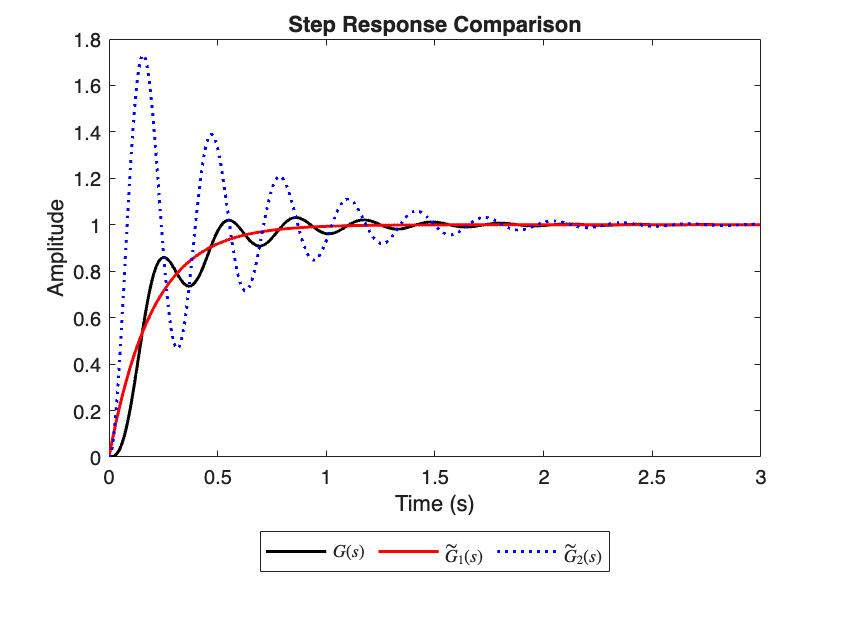
Settling time estimation For \(G(s)\), the settling time is estimated as the value of \(t\) permanently enters the interval \([0.99, 1.01]\). For \(\tilde{G}_1(s)\) and \(\tilde{G}_2(s)\), the settling time is approximated with the formula \(T_{99\%} = \frac{5}{\gamma}\) and \(T_{99\%} = \frac{5}{\alpha}\), respectively (see Useful formulas).

Show code cell source

Hide code cell source

idx = max(find(y < 0.99, 1, 'last'), find(y > 1.01, 1, 'last'));
T_G = t(idx);
T_G1 = 5 / gamma;
T_G2 = 5 / alpha;

disp(sprintf('\nSettling time (99 percent):\n\tof G(s): %.2f sec\n\tof G1(s): %.2f sec\n\tof G2(s): %.2f sec\n', T_G, T_G1, T_G2));

Settling time (99 percent):
	of G(s): 1.51 sec
	of G1(s): 1.00 sec
	of G2(s): 2.50 sec