Solutions of Exercise 5.3

Fig. 53 Block diagram of the control system

The proportional feedback controller \(F(s) = 4\) was designed assuming that the system \(G^0(s)\) was identical to the model, \(G(s) = \frac{1}{s(s+1)}\).

The real system, however, is

\[ G^0(s) = G(s) \frac{\alpha}{s+\alpha}, \quad \text{where } \alpha > 0 \]

The control loop is closed as in Fig. 53.

1. Compute the real closed-loop transfer function \(G_c^0(s)\), and use the Routh-Hurwitz criterion to establish for what values of \(\alpha\) this transfer function is stable.

2. Find the multiplicative uncertainty \(\Delta(s)\) that captures the plant-model mismatch.

3. Using the Bode plot of the nominal complementary sensitivity \(T(s)\) in Fig. 54, apply the “Criterion for robustness to model mismatch” (Criterion 6.2) to find for what values of \(\alpha\) the robustness can be guaranteed.

4. Comment the (possible) differences in the solutions to question 1 and question 3.

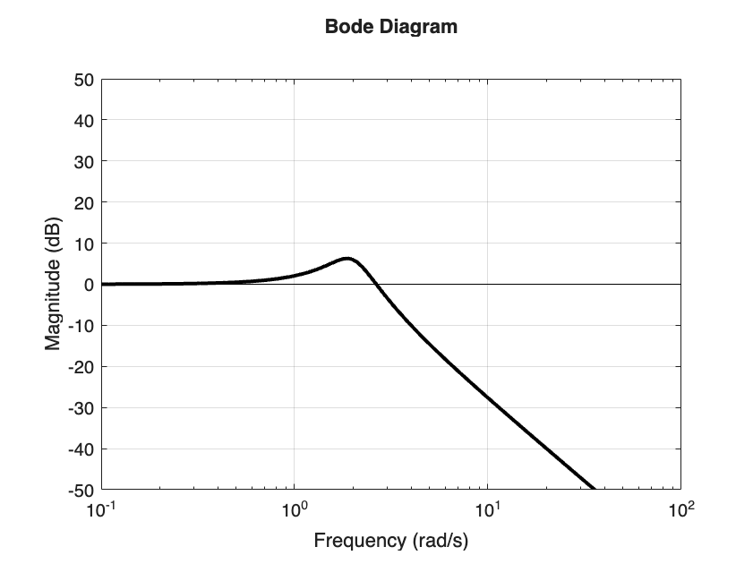
Fig. 54 Magnitude Bode plot of the nominal complementary sensitivity transfer function \(T(s)\).

---

Solution

Question 1

To compute the real closed-loop transfer function, we start by computing the real open-loop one:

\[ G_o^0(s) = F(s) G^0(s) = 4 \frac{1}{s(s+1)} \frac{\alpha}{s + \alpha} = \frac{4\alpha}{s(s+1)(s+\alpha)} \]

The real closed-loop transfer function is then

\[ G_c^0(s) = \frac{G_o^0(s)}{1+G^0_o(s)} = \frac{4 \alpha}{s^3 + (\alpha + 1) s^2 + \alpha s + 4 \alpha} \]

Because it’s a third-order system, the poles cannot be explicitly computed. We therefore use the Routh-Hurwitz criterion on the characterist polynomial

\[ \Phi(s) = s^3 + (\alpha + 1) s^2 + \alpha s + 4 \alpha \]

The Routh table reads

\( \begin{array}{cc} 1 & \alpha \\ \alpha + 1 & 4 \alpha \\ \hline c_0 \\ d_0 \end{array} \qquad \text{ where } c_0 = \frac{\alpha(\alpha + 1) - 4\alpha}{\alpha + 1} = \frac{\alpha^2 - 3\alpha}{\alpha + 1} \text{ and } d_0 = \frac{c_0 \cdot 4\alpha}{c_0} = 4 \alpha \)

We then set all the elements of the first column to be positive

(20)\[\begin{split} \begin{dcases} 1 > 0 & \\ \alpha + 1 > 0 & \\ \frac{\alpha^2 - 3 \alpha}{\alpha + 1} > 0 \quad & \text{(C)}\\ 4 \alpha > 0 & \end{dcases} \end{split}\]

To solve inequality (C), we apply the rule of signs by understanding when the numberator and denominator are both positive/negative

Numerator > 0 gives: $\( \alpha^2 - 3 \alpha > 0 \qquad \Rightarrow \qquad \alpha < 0 \cup \alpha > 3 \)$

Denominator > 0 gives: $\( \alpha > -1 \)$

Then we get the following table, from which it is evident that the solution is \(-1 < \alpha < 0 \cup \alpha > 3\). The first interval needs to be discarded, because according to the text of the exercise \(\alpha\) must be positive.

Reconstructing (20) we get

\[\begin{split} \begin{dcases} \forall \alpha \\ \alpha > -1 \\ \alpha > 3 \quad & \text{(C)} \\ \alpha > 0 \end{dcases} \end{split}\]

The solutions is \(\boxed{\alpha > 3}\).

Question 2

The multiplicative uncertainty \(\Delta(s)\) is such that

\[ G^0(s) = G(s) \left( 1 + \Delta(s) \right) \]

Replacing the definition of \(G^0(s)\) and \(G(s)\) we get

\[ \cancel{\frac{1}{s(s+1)}} \frac{\alpha}{s+\alpha} = \cancel{\frac{1}{s(s+1)}} \left( 1 + \Delta(s) \right) \]

Isolating \(\Delta(s)\), we get

\[ \Delta(s) = \frac{\alpha}{s+\alpha} - 1 = \boxed{-\frac{s}{s+\alpha}} \]

Question 3

To apply the Robustness Criterion, we need to plot \(\lvert \Delta(i \omega) \lvert_{\text{dB}}\) and then mirror it with respect to the 0dB axis to get \(-\lvert \Delta(i \omega) \lvert_{\text{dB}}\).

The (asymptotic) Bode plot we note that

• \(\Delta(s)\) has a zero in \(s = 0\), so the initial slope will be \(+20\) dB/decade;

• \(\Delta(s)\) has a pole in \(s=-\alpha\), therefore for \(\omega > \alpha\) the asymptotic magnitude plot will be flat (\(0\) dB/decade)

• \(\lim_{s \to \infty} \lvert \Delta(s) \lvert = 1 = 0\) dB

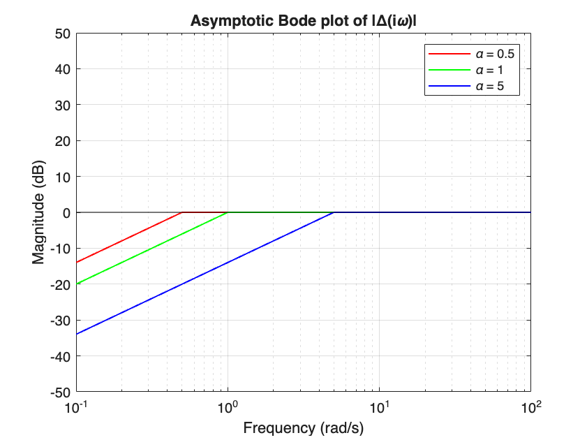
Fig. 55 Asymoptotic magnitude plot of \(\Delta(s)\) for several values of \(\alpha\).

Let’s now sketch \(-\lvert \Delta(i \omega)\lvert_{\text{dB}}\) on top of Fig. 54

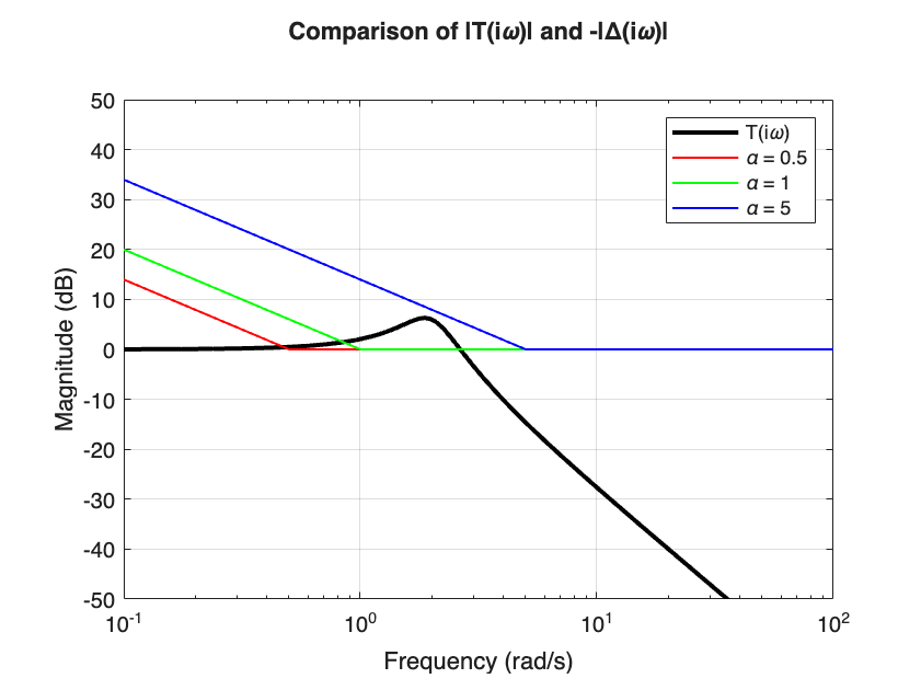
Fig. 56 Comparison between the nominal complementary sensitivity \(\lvert T(i \omega) \lvert_{\text{dB}}\) and \(-\lvert \Delta(i \omega) \lvert_{\text{dB}}\)

We can clearly see that for \(\alpha = 0.5\) and \(\alpha = 1\) the plot \(-\lvert \Delta(i \omega) \lvert_{\text{dB}}\) is not always higher than \(\lvert T(i \omega) \lvert_{\text{dB}}\). For \(\alpha = 5\), instead, there is still some room for (\(-\lvert \Delta(i \omega) \lvert_{\text{dB}}\) is not tangent!). Let’s try to reduce \(\alpha\) to \(4\).

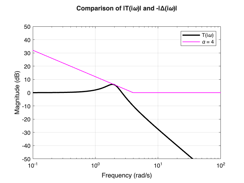
Fig. 57 Comparison between the nominal complementary sensitivity \(\lvert T(i \omega) \lvert_{\text{dB}}\) and \(-\lvert \Delta(i \omega) \lvert_{\text{dB}}\) for \(\alpha=4\).

From here, we can see that robust closed-loop stability is achieved for any \(\boxed{\alpha > 4}\)

Question 4

There is, indeed, a difference between the solution of Question 1 (\(\alpha > 3\)) and the solution of Question 3 (\(\alpha > 4\)). The reason for this difference is that Criterion 6.2 is only a sufficient condition. This means that:

• If Criterion 6.2 is satisfied, than robust closed-loop stability is guaranteed;

• If Criterion 6.2 is violated, we can not exclude closed-loop stability.

In other words, Criterion 6.2 is conservative and does not entitle us to claim that the real closed-loop is unstable for \(\alpha < 4\).