Solutions of Exercise 5.2

Fig. 46 Block diagram of the control system

The controller \(F(s) = \frac{s+10}{s}\) was designed assuming that the system \(G^0(s)\) was identical to the model \(G(s) = \frac{1}{s+10}\). In Fig. 47, the nominal open-loop transfer function \(G_o(s) = F(s) \cdot G(s)\).

1. Sketch the nominal complementary sensitivity function \(T(s)\) using the sketching rules discussed in Lecture F7.

Unfortunately, there’s a mismatch between the real system \(G^0(s)\) and its model \(G(s)\). In fact

\[ G^0(s) = G(s) \left( 1 + \Delta(s) \right) \]

where the multiplicative uncertainty \(\Delta(s)\) does not have any pole in the right-hand half plane, but is not known. We know, however, an upper bound for its amplitude

(19)\[ \lvert \Delta(i \omega) \lvert \leq \frac{0.9}{\sqrt{1 + \omega^2}} = \left\lvert \frac{0.9}{1 + i \omega} \right\lvert \]

2. Does the feedback controller \(F(s)\), implemented as in Fig. 46, guarentee the closed-loop stability for \(G^0(s)\) despite the uncertainty?

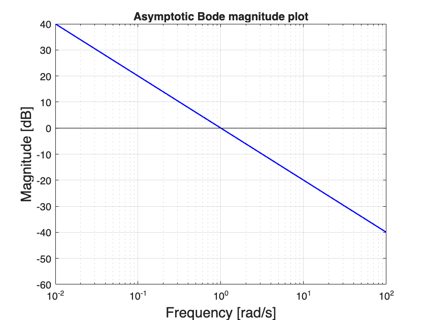
Fig. 47 Magnitude Bode plot of the nominal open-loop transfer function \(G_o(s)\).

---

Solution

Question 1

The nominal complementary sensitivity transfer function \(T(s)\) is defined as

\[ T(s) = \frac{G_o(s)}{1 + G_o(s)}, \]

where \(G_o(s)\) is the nominal open-loop transfer function (mind the difference between \(G_o(s)\) and $G^0(s), they are two different things!).

To sketch \(\lvert T(i \omega) \lvert_{\text{dB}}\) we use the rule (14). By sketching it on top of Fig. 47 we get

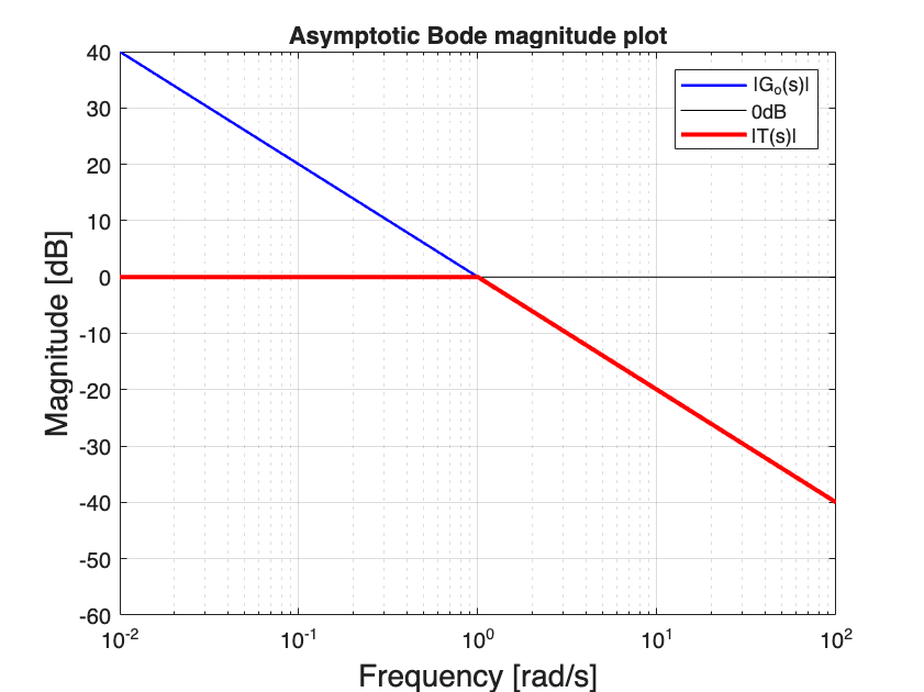
Fig. 48 Sketch of the nominal complementary sensitivity function’s bode plot.

Question 2

The ancillary assumptions of Criterion 6.2 (Criterion for robustness to model mismatch) are satisfied. To verify whether \(F(s)\) guarantees the closed-loop stability for the real system \(G^0(s)\), we need to:

• Sketch \(\lvert \Delta(i \omega) \lvert_{\text{dB}}\)

• Mirror it with respect to the 0dB axis to get \(-\lvert \Delta(i \omega) \lvert_{\text{dB}}\)

• Verify that \(\lvert T(i \omega)\lvert_{\text{dB}} < -\lvert \Delta(i \omega) \lvert_{\text{dB}}\)

Note that (19) represents the magnitude \(\frac{0.9}{1+s}\). Therefore its magnitude Bode plot will be flat at \(20 \log_{10}(0.9) = -1\) dB for \(\omega < 1\) rad/s, after which it decreases with a slope \(-20\) dB/decade.

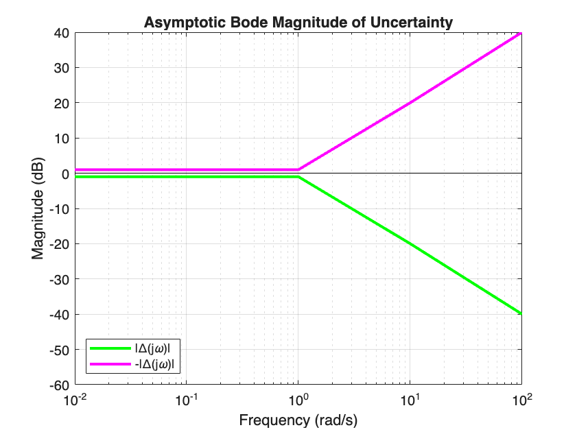
Fig. 49 Sketch of the magnitude plot of \(\Delta(i \omega)\).

Now we can compare \(\lvert T(i \omega) \lvert_{\text{dB}}\) to \(-\lvert \Delta (i \omega) \lvert_{\text{dB}}\), to make sure the former is always smaller than the latter.

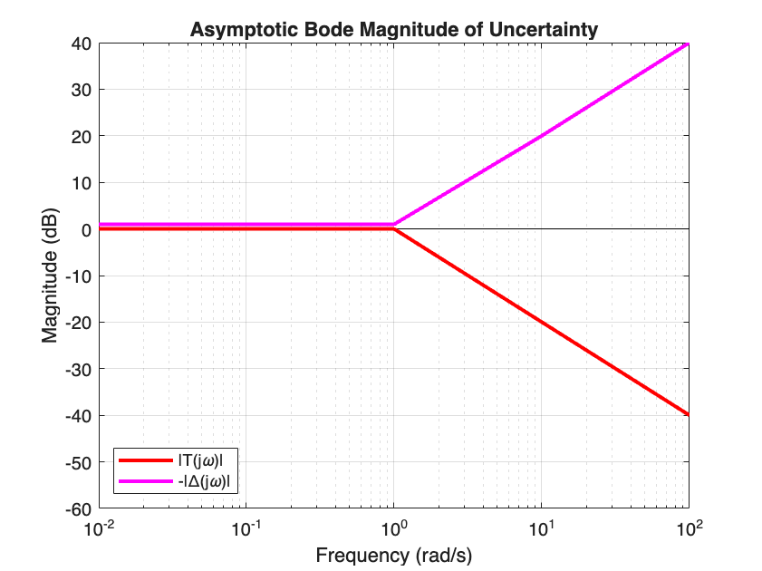
Fig. 50 Comparison between \(\lvert T(i \omega) \lvert_{\text{dB}}\) and \(-\lvert \Delta(i \omega) \lvert_{\text{dB}}\).

As we can see, the condition is satisfied at every frequency \(\omega\). Therefore, the robust closed-loop stability can be guaranteed.

Note

In this exercise, we used an asymptotic approximation of the complementary sensitivity function (Equation (14)). This approximation is sufficient when the exact plot of \(\lvert T(i \omega) \vert\) is not available.

In practical applications, however, you should use the exact magnitude \(\lvert T(i \omega) \lvert\) whenever it is available, rather than relying on the asymptotic approximation.

Warning

If \(\lvert T(i \omega)\lvert_{\text{dB}}\) is higher than \(-\lvert \Delta (i \omega) \lvert_{\text{dB}}\), even in a narrow range of frequencies, robust closed-loop stability could not be guaranteed!