Solutions of Exercise 5.0

Solutions of Exercise 5.0#

Consider the control system in Fig. 32, where $n(t)$ is the sinusoidal measurement noise $n(t) = \sin(50 t)$.

../_images/ex0-block.svg — Fig. 32 Block diagram of the control system#

Assume that $F(s)=1$. How much is the closed-loop attenuating the measurement noise?
Design a proportional controller $F(s) = K$, with $K >0$, that achieves a measurement noise attenuation factor of $10$.

3. Bonus

Design $F(s)=\frac{\alpha}{s + \alpha}$, with $\alpha > 0$, such that

The crossover frequency is at least $10$ rad/s
The phase margin is at least $50^\circ$
The attenuation factor is $10$

Tip

Based on the Bode plot of $G(s)$ reported in Fig. 33, sketch the complementary sensitivity function’s magnitude plot.

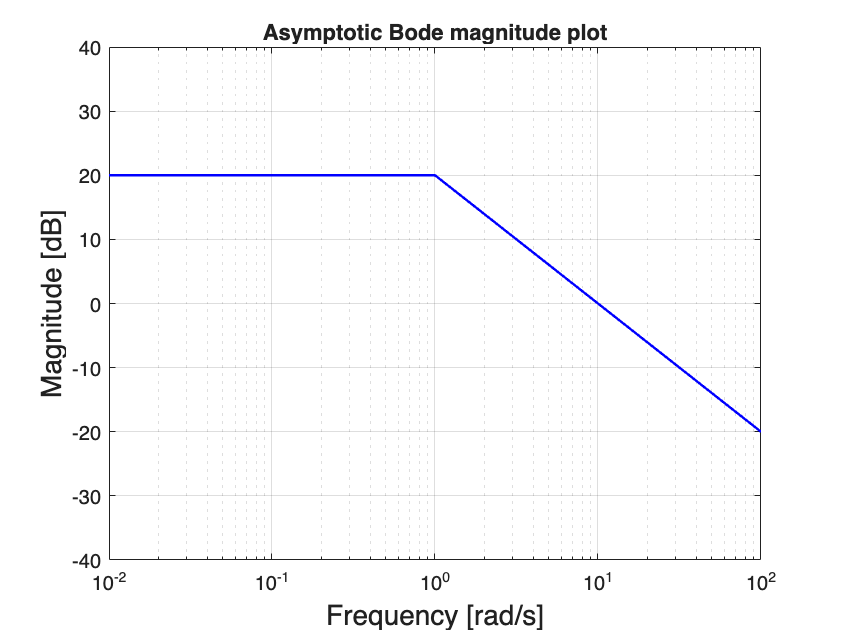
../_images/e9279328077340ca75ddff51d8d2c348d3eb7ef5fa9e7369ba1630e07665fdf9.png — Fig. 33 Magnitude Bode plot of $G(s)$#

Solution#

From Lecture 7, we know that the transfer function between the noise $N(s)$ and the output $Y(s)$ is the complementary sensitivity function $T(s)$

\[ T(s) \equiv \frac{Y(s)}{N(s)} = - \frac{F(s)G(s)}{1+ F(s)G(s)} \]

For proportional controllers $F(s) = K$, replacing $G(s)$ we get

\[ T(s) = -\frac{K \frac{10}{s+1}}{1 + K \frac{10}{s+1}} = -\frac{10 K}{s + 10K + 1} \]

We can also sketch the asymptotic magnitude Bode plot of $T(s)$ using the rule

(14)#\[\begin{split} \lvert T(i \omega) \lvert_{\text{dB}} \approx \begin{dcases} 0 \text{ dB } & \text{where } \lvert G_o (i \omega)\lvert_{\text{dB}} > 0dB \\ \lvert G_o(i \omega) \lvert_{\text{dB}} & \text{where } \lvert G_o (i \omega)\lvert_{\text{dB}} < 0dB \end{dcases} \end{split}\]

Since $T(s)$ is stable for any $K>0$, the effect of $n(t) = \sin(50t)$ on the output $y(t)$ is described by $\lvert T(i50) \lvert$. In particular, the attenuation factor is defined as $\frac{1}{\lvert T(i50) \lvert}$.

There are two ways to compute $\lvert T(i50) \lvert$. We will start from the approach based on Bode plot for both Question 1 and 2, as it is simpler, and then embark in the analytical solution.

Question 1#

We can easily compute $\lvert T(i 50) \lvert_{\text{dB}}$ using the sketching rule (14). Note that in this case we do have the Bode plot of $\lvert G_o(i \omega) \lvert$: it is the same as the Bode plot og $G(i \omega)$ because $K=1$.

Doing so, we obtain the Bode plot in Fig. 34.

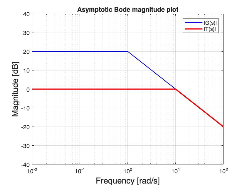
../_images/b26a5510b099f56c74fe54c6985b2fcc890b6f6623ad64a125c87793a026b768.png — Fig. 34 Magnitude Bode plot of $G_o(s)= G(s)$ and $T(s) for $K=1$#

From this, we can note that $\lvert T(i 50) \lvert_{\text{dB}} \approx -13$ dB or, equivalently, $\lvert T(i 50) \lvert = 10^{\frac{-13}{20}} \approx 0.22$.

This means that a sinusoidal measurement noise with amplitude $1$ at $50$ rad/s will cause the output to oscillate with amplitude $0.22$ at the same frequency. In this case, we say that the measurement noise is attenuated by a factor $\frac{1}{0.22} \approx 4.5$.

Question 2#

Let’s sart by observing that an attenuation factor of $10$ corresponds to $\lvert T(i 50) \lvert_{dB }= -20$ dB. From the sketch of complementary sensitivity for $K=1$ in Fig. 34, we can note that

$\lvert T(i 50) \lvert_{\text{dB}} = - 13$ dB
The current crossover frequency is $\omega_c = 10$ rad/s, which is smaller than the noise of the measuement noise ($50$ rad/s).

Because $50 > \omega_c$, $\lvert T(i 50) \lvert_{\text{dB}} = \lvert G_o(i 50) \lvert_{\text{dB}} = \lvert K \lvert_{dB} + \lvert G(i 50) \lvert_{dB} = \lvert K \lvert_{dB} - 13$ dB.

To reduce it to $-20$ dB, it is enough to select $\lvert K \lvert_{\text{dB}} = -7$ dB, that is, $\boxed{K = 10^{\frac{-7}{20}} = 0.44}$.

We can double-check this result, by sketching $\lvert T(i \omega) \lvert_{\text{dB}}$ as follows:

Sketch $\lvert G_o(i \omega) \lvert_{\text{dB}}$ by moving decreasing the Bode plot of $G(s)$ by $7$ dB.
Apply (14) with this $\lvert G_o(i \omega) \lvert_{\text{dB}}$.

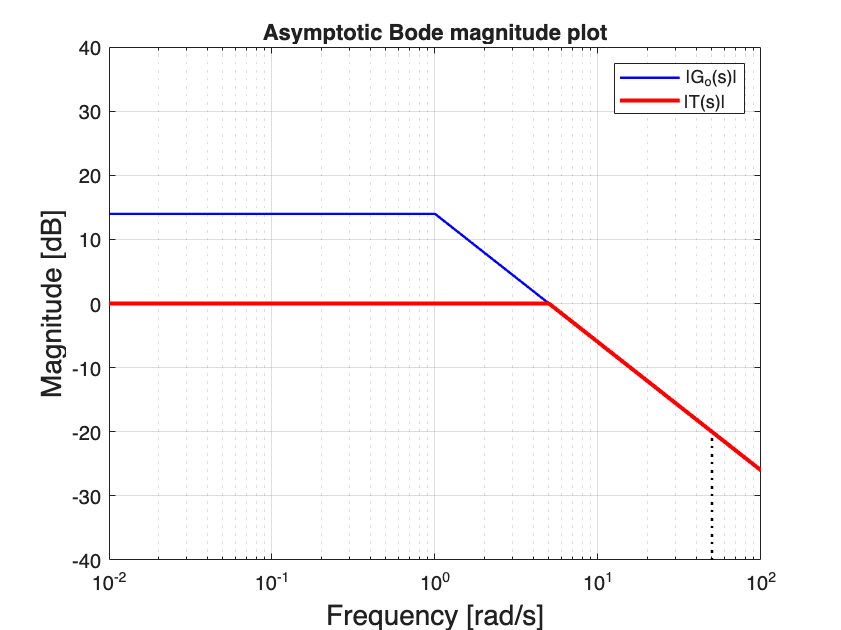
../_images/b939c18c9f07a1df39bc2b8ef595d547507f4d1fe7af541e3f54174a48644230.png — Fig. 35 Magnitude Bode plot of $G_o(s)= G(s)$ and $T(s)$ for $K=0.44$#

Note that any $\boxed{0 < K \leq 0.44}$ works, since decreasing $K$ will cause $\lvert G_o(i \omega) \lvert_{\text{dB}}$ to move further down.

The price for attenuation

As you can easily note in the plot below, the price of this increased attenuation is the halving of the crossover frequency (and, hence, of the closed-loop bandwidth)!

Analytical solutions#

Let us derive the analytical expression of the complementary sensitivity at $50$ rad/s, as a function of the proportional controller gain $K$:

\[ \lvert T(i50) \lvert = \left\lvert \frac{10K}{i 50 + 10K +1} \right\lvert = \left\lvert \frac{10K}{10K +1 + i50}\cdot\frac{10K + 1 - i50}{10 K + 1 - i50} \right\lvert = \left\lvert \frac{100K^2 + 10K - i500K}{(10K +1)^2 + 50^2}\right\lvert \]

We now isolate the real part from the imaginary part

\[ \lvert T(i50) \lvert = \left\lvert \frac{100K^2 + 10K}{(10K +1)^2 + 50^2} - i \frac{500K}{(10K +1)^2 + 50^2} \right\lvert \]

The modulus is then

(15)#\[ \lvert T(i50) \lvert = \sqrt{\left( \frac{100K^2 + 10K}{(10K +1)^2 + 50^2} \right)^2 + \left( \frac{500K}{(10K +1)^2 + 50^2} \right)^2} \]

Question 1 - $K=1$#

To solve Question 1, we just replace $K=1$ in (15). Doing so, we obtain:

\[ \lvert T(i 50) \lvert = \sqrt{\left(\frac{110}{2621} \right)^2 + \left( \frac{500}{2621} \right)^2 } \approx 0.2 \]

This corresponds to an attenuation factor of $\frac{1}{0.2} \approx 5$.

Question 2#

We need to compute for what values of $K$ (15) is smaller than $0.1$, so that the attenuation factor is (at least) $10$. This inequality is really nasty, because if we try to evaluate the squares a fourth order term $K^4$ appears. Instead of solving it explicitly, we can try probing different values of $K$ to numerically find one that makes $\lvert T(i 50) \lvert \approx 0.1$. Note that the calculation of $\lvert T(i 50) \lvert$ for different values of $K$ can be easily automated with a programmable calculator!

function print_modulus_T(K)
    term_1 = (100*K^2 + 10*K) / ((10*K+1)^2 +50^2);
    term_2 =500*K / ((10*K+1)^2 +50^2);
    T = sqrt(term_1^2 + term_2^2);
    disp(sprintf('For K=%.2f\t|T(i50)| = %.3f\n', K, T));
end

print_modulus_T(1);
print_modulus_T(0.1);
print_modulus_T(0.5);

For K=1.00	|T(i50)| = 0.195

For K=0.10	|T(i50)| = 0.020

For K=0.50	|T(i50)| = 0.099

Bingo! From here, we can deduce $K=0.5$ satisfies the requirement

Warning

This numerical method does not guarantee that any $K < 0.5$ satisfies the requirement!

Question 3#

We now use the controller $F(s) = \frac{\alpha}{s + \alpha}$. Let’s start by noting that the static gain of this controller is $1$. In fact, it can be re-written as

\[ F(s) = \frac{1}{\tau s + 1} \quad \text{where } \tau = \frac{1}{\alpha} \]

The Bode plot of the open-loop transfer function $G_o(s)$ will be the same as $G(s)$ for $\omega < - \alpha$. After the pole in $s = - \alpha$, its slope will decrease by an additional $-20$ dB/decade.

This additional negative slope is really useful for reducing the effect of measurement noise at frequencies higher than $\alpha$, as $\lvert T(i \omega) \lvert_{\text{dB}}$ will be even lower, thereby attenuating the effect of high-frequency noise. Let’s go for $\alpha = 10$, plotting $\lvert G_o(i \omega) \lvert_{\text{dB}}$ and the corresponding $\lvert T(i \omega) \lvert_{\text{dB}}$ obtained with the approximation (14)

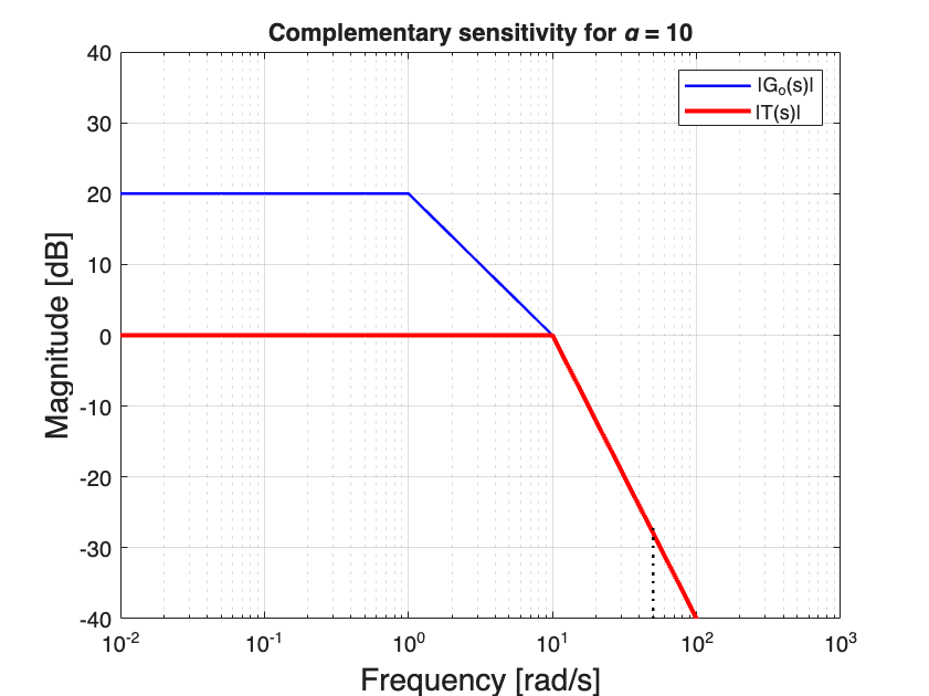
../_images/482c96ec59ac35ac7062a2a152307494e4ca8e581d8d81d2917353c22315a8be.png — Fig. 36 Magnitude Bode plot of $G_o(s)= \frac{\alpha}{s + \alpha} G(s)$ and $T(s)$ for $\alpha = 10$#

With this choice:

$\omega_c \approx 10$ rad/s, because $G_o(s)$ crosses the 0dB axis at 10 rad/s.
$\lvert T(i50) \lvert_{\text{dB}} \approx -26$ dB, so the attenuation factor will be $\frac{1}{10^{\frac{\lvert T(i50) \lvert_{\text{dB}}}{20}}} = 10^{\frac{26}{20}} = 20 > 10$.

We just have to check that the phase margin is larger than $50^\circ$:

\[ \varphi_m = 180 + \angle G_o(i \omega_c) = 180 - \textrm{atan} \left( \frac{\omega_c}{1} \right) - \textrm{atan} \left( \frac{\omega_c}{\alpha} \right) \]

For $\omega_c = 10$ rad/s and $\alpha = 10$ the phase margin is $39^\circ$. This is insufficient!

Let’s now try with $\alpha = 20$.

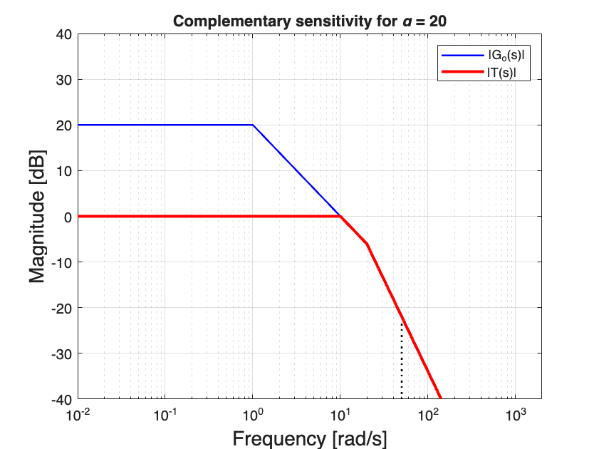
../_images/e689629c2cd86303bb5ea6f632f76a805bceebe90f9c70eb8a6cbcbc56720ca9.png — Fig. 37 Magnitude Bode plot of $G_o(s)= \frac{\alpha}{s + \alpha} G(s)$ and $T(s)$ for $\alpha = 20$#

Now:

The crossover frequency is still $\omega_c \approx 10$ rad/s
$\lvert T(i50) \lvert_{\text{dB}} \approx -23$ dB, so the attenuation factor will be $\frac{1}{10^{\frac{\lvert T(i50) \lvert_{\text{dB}}}{20}}} = 10^{\frac{23}{20}} = 12.5 > 10$.
The phase margin is $\varphi_m \approx 57^\circ$ which is larger than what we needed!

What’s the catch?

This controller allows to achieve much better disturbance compensation with a larger bandwidth compared to Fig. 35, at the price of a smaller phase margin (and hence, slightly larger closed-loop oscillations).

With the controller designed in Fig. 35, the phase margin was approximately $90^\circ$!

Step response simulations#

We can illustrate this trade-off by simply simulating the closed-loop acheived by $F(s) = 0.44$ and by $F(s) = \frac{20}{s + 20}$, when

$r(t) = \text{step}(t)$, and
$n(t) = \sin(50t)$

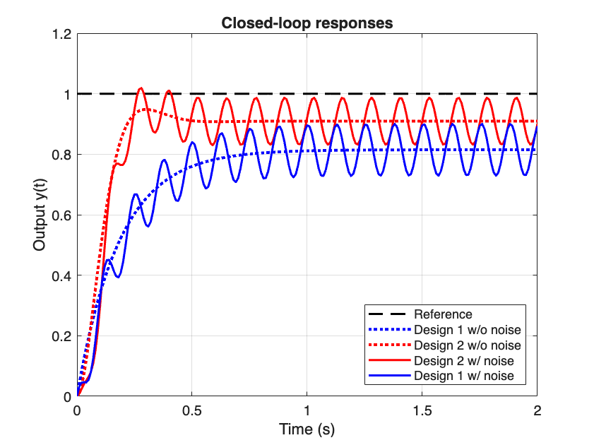
../_images/3386c3a6435247f89dab357f2260f3429c76fd5a8ccac72f9619939297abf731.png — Fig. 38 Closed-loop step response for design 1 ($F(s)=0.44$) and design 2 ($F(s) = \frac{\alpha}{s + \alpha}$) with and without the noise $n(t).$#

Solutions of Exercise 5.0

Contents

Solutions of Exercise 5.0#

Solution#

Question 1#

Question 2#

Analytical solutions#

Question 1 - \(K=1\)#

Question 2#

Question 3#

Step response simulations#