Plotting the exact Sensitivity function

In case you are curious, below you can find the code to plot the exact sensitivity transfer function.

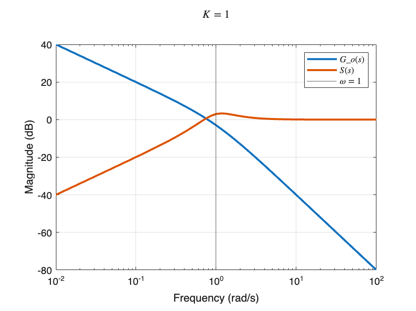
\(K = 1\)

s = tf('s');
K = 1;
Go = K / (s * (s+1));
S = 1 / (1 + Go);
figure; 
bodemag(Go);
hold on; grid on;
bodemag(S);
xline(1);
legend('$G_o(s)$', '$S(s)$', '$\omega=1$', 'Interpreter', 'latex');
title('$K = 1$', 'Interpreter', 'latex')

\(K = 1 + \sqrt{5}\)

Let’s now plot the open-loop transfer function and the sensitivity function for \(K= 1 + \sqrt{161}\), which was the analytical solution we got.

K = 1 + sqrt(161);
G = K / (s * (s+1));
S = 1 / (1 + G);
figure; 
bodemag(G);
hold on; grid on;
bodemag(S);
xline(1);
legend('$G_o(s)$', '$S(s)$', '$\omega=1$', 'Interpreter', 'latex');
title('$K = 1 + \sqrt{5}$', 'Interpreter', 'latex')

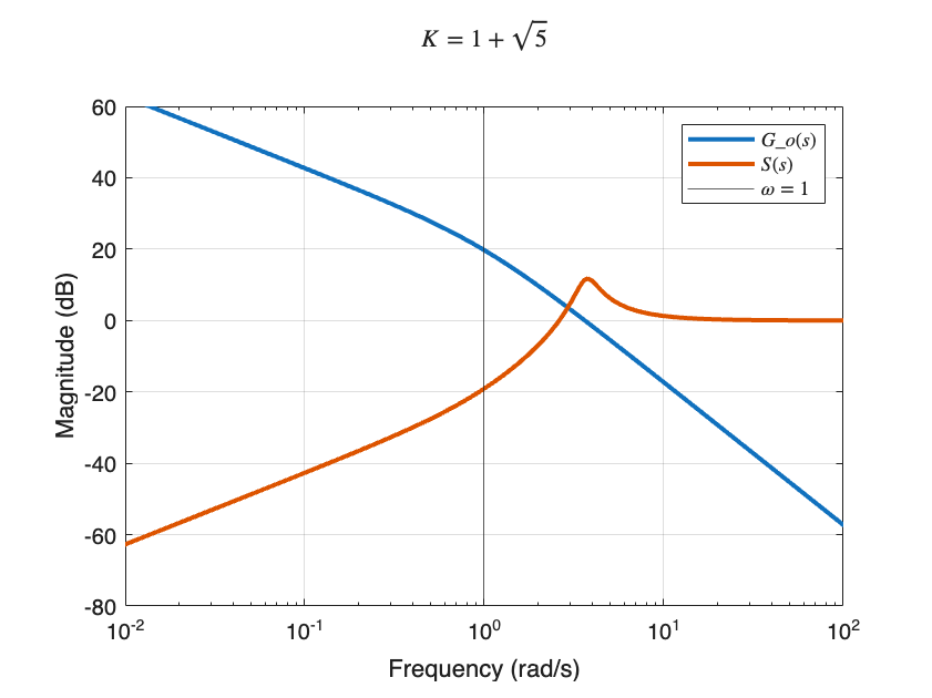
As you can see, \(\lvert S(i 1) \lvert_\text{dB} = -19\) dB! Let’s triple-check by printing this value:

S_mag = abs(freqresp(S, 1));
S_mag_db = 20 * log10(S_mag)

S_mag_db = -19.0849